
Coax to waveguide#
This notebook outlines the design and simulation workflow for a horn antenna fed by a standard WR-90 waveguide operating at a target frequency of 10 GHz (λ≈30mm)
Design Parameters#
The antenna geometry and probe feed are defined based on the following physical constraints:
Waveguide (WR-90):
22.86 mm (width)
10.16 mm (height)
40 mm (length)
Probe Feed:
Probe Length: 5.89 mm (≈λ/5) to ensure optimal impedance matching.
Coaxial Geometry: 3.6 mm (outer diameter) and 1.28 mm (inner diameter).
These parameters serve as the foundation for our geometric construction and subsequent discretization, ensuring the antenna is tuned for its intended frequency of operation.
import gmsh
import math
import os
import json

from palacetoolkit.viz import view_mesh
from palacetoolkit.geometry import extract_tag, xmin, xmax, ymin, ymax, zmin, zmax
from palacetoolkit.mesh import create_graded_mesh, run_for_docs
from palacetoolkit.viz import view_mesh
from palacetoolkit.mesh import (
    create_graded_mesh
)
Parameters:#
inner_diameter_mm: Inner diameter of the coaxial cable in millimeters.
outer_diameter_mm: Outer diameter of the coaxial cable in millimeters.
probe_length_mm : Length of the probe in milimiters.
length_mm: Length of the coaxial cable section in millimeters.
wg_height: Height of the rectangular waveguide in millimeters.
wg_length: Length of the rectangular waveguide in millimeters.
wg_width: Width of the rectangular waveguide in millimeters.
freq_ghz: Frequency of the wave in gigahertz.
verbose: Verbosity level for Gmsh output
filename: Name of the output mesh file.
inner_diameter_mm: float = 1.28
outer_diameter_mm: float = 3.6
probe_length_mm = 5.89
length_mm: float = 5
wg_height: float = 10.16
wg_length: float = 40
wg_width: float = 22.86
freq_ghz: float = 10.0
verbose: int = 2
filename: str = "coax_to_waveguide.msh"
mesh_order = 1
gui = False
order = 1
Initializing the Modeling Environment#
gmsh.initialize()
gmsh.option.setNumber("General.Verbosity", 5)
gmsh.model.add("coax_to_waveguide")
kernel = gmsh.model.occ
Design Parameter Calculation#
We calculate the operating wavelength (λ) and derive the critical dimensions for the coaxial probe and backshort position. By basing these values on the 10 GHz design frequency, we ensure the geometry is physically optimized for efficient power transfer within the waveguide structure.
c = 3e8
lamda = (c / (freq_ghz * 1e9)) * 1e3

inner_radius = inner_diameter_mm / 2
outer_radius = outer_diameter_mm / 2

# y_top is the y-coordinate of the center of the coax probe,
# which is typically placed at the center of the waveguide height
y_top = wg_height / 2
coax_y_max = y_top + length_mm

# backshort_z is the distance from the probe tip to the backshort plane,
# which is typically around λ/5 for good impedance matching
backshort_z = lamda / 5

print(f"Wavelength:           {lamda:.2f} mm")
print(f"Probe length:   {probe_length_mm:.2f} mm")
print(f"Backshort Z position: {backshort_z:.2f} mm")
Wavelength:           30.00 mm
Probe length:   5.89 mm
Backshort Z position: 6.00 mm
Geometry Construction and Boolean Operations#
In this step, we construct the CAD model by defining the waveguide box and the coaxial feed components. We use Boolean cut operations to integrate the probe into the waveguide and define the dielectric region. Finally, we perform a global fragment operation to ensure all geometric volumes are properly connected, forming a unified topology ready for discretization.
# Waveguide box
waveguide = kernel.addBox(
    -wg_width/2, -wg_height/2, 0,
        wg_width,    wg_height,   wg_length
)

# Outer coax cylinder
outer_cyl = kernel.addCylinder(0, y_top, backshort_z,
                                0, length_mm, 0, outer_radius)

# Inner conductor
inner_cyl = kernel.addCylinder(0, coax_y_max, backshort_z,
                                0, -(length_mm + probe_length_mm), 0, inner_radius)

kernel.synchronize()

coax_dielectric, _ = kernel.cut([(3, outer_cyl)], [(3, inner_cyl)],
                                removeObject=True, removeTool=False)

waveguide_cut, _ = kernel.cut([(3, waveguide)], [(3, inner_cyl)],
                                removeObject=True, removeTool= True)

kernel.synchronize()

all_volumes = gmsh.model.getEntities(3)
kernel.fragment(all_volumes, [])
kernel.synchronize()
Info    : [  0%] Difference
Info    : [ 10%] Difference
Info    : [ 20%] Difference
Info    : [ 30%] Difference
Info    : [ 40%] Difference
Info    : [ 50%] Difference
Info    : [ 60%] Difference
Info    : [ 70%] Difference - Filling splits of edges
Info    : [ 80%] Difference - Making faces
Info    : [ 90%] Difference - Classify solids
Info    : [  0%] Difference
Info    : [ 10%] Difference
Info    : [ 20%] Difference
Info    : [ 30%] Difference
Info    : [ 70%] Difference
Info    : [ 80%] Difference
Info    : [ 90%] Difference

Info    : [  0%] Fragments
Info    : [ 10%] Fragments
Info    : [ 20%] Fragments
Info    : [ 30%] Fragments
Info    : [ 40%] Fragments
Info    : [ 50%] Fragments
Info    : [ 60%] Fragments
Info    : [ 70%] Fragments
Info    : [ 80%] Fragments - Adding holes
Info    : [ 90%] Fragments
Geometric Entity Classification#
Here, we categorize the fragmented CAD entities into functional groups based on their spatial coordinates. We define logical filters to isolate the waveguide walls, coaxial conductors, waveports, and internal volumes. This classification step is essential for mapping the geometry to the specific physical boundary conditions required by the Palace solver
all_2d_entities = gmsh.model.getEntities(2)
all_3d_entities = gmsh.model.getEntities(3)

def is_interface(x):
    return (math.isclose(ymin(x), y_top, abs_tol=1e-4) and
            math.isclose(ymax(x), y_top, abs_tol=1e-4) and
            math.isclose(xmax(x), outer_radius, abs_tol=1e-4))

def is_coax_port(x):
    return (math.isclose(ymin(x), coax_y_max, abs_tol=1e-4) and
            math.isclose(ymax(x), coax_y_max, abs_tol=1e-4) and
            math.isclose(xmax(x), outer_radius, abs_tol=1e-4))

def is_inner_conductor(x):
    return (math.isclose(xmax(x), inner_radius, abs_tol=1e-4) and
            not is_interface(x))

def is_outer_conductor(x):
    return (math.isclose(xmax(x), outer_radius, abs_tol=1e-4) and
            ymin(x) >= y_top - 1e-4 and
            not is_coax_port(x) and
            not is_interface(x))

def is_waveport(x):
    return( math.isclose(zmax(x), wg_length, abs_tol=1e-4) and
            math.isclose(zmin(x), wg_length, abs_tol=1e-4))

def is_waveguide_wall(x):
    return (not is_coax_port(x) and
            not is_inner_conductor(x) and
            not is_outer_conductor(x) and
            not is_waveport(x) and
            not is_interface(x))

def is_coax_volume(x):
    return ymin(x) >= y_top - 1e-4

def is_waveguide_volume(x):
    return ymax(x) <= y_top + 1e-4

coax_port_surfs      = [x for x in all_2d_entities if is_coax_port(x)]
inner_cond_surfs     = [x for x in all_2d_entities if is_inner_conductor(x)]
outer_cond_surfs     = [x for x in all_2d_entities if is_outer_conductor(x)]
waveguide_wall_surfs = [x for x in all_2d_entities if is_waveguide_wall(x)]
waveport_surfs       = [x for x in all_2d_entities if is_waveport(x)]
coax_vols      = [x for x in all_3d_entities if is_coax_volume(x)]
waveguide_vols = [x for x in all_3d_entities if is_waveguide_volume(x)]
Physical Group Assignment#
In this block, we map the classified geometric entities to Physical Groups. Assigning these unique identifiers allows the Palace solver to distinguish between different materials and boundary conditions, such as the waveguide walls (PEC), the coaxial probe, and the internal air and dielectric volumes. Finally, we store these identifiers in a pg_map dictionary for streamlined reference during the simulation configuration.
pg_coax_port = gmsh.model.addPhysicalGroup(2, [x[1] for x in coax_port_surfs], -1, "coax_port")
pg_probe = gmsh.model.addPhysicalGroup(2, [x[1] for x in inner_cond_surfs], -1, "inner_conductor")
pg_outer_cyl = gmsh.model.addPhysicalGroup(2, [x[1] for x in outer_cond_surfs], -1, "outer_conductor")
pg_waveguide = gmsh.model.addPhysicalGroup(2, [x[1] for x in waveguide_wall_surfs], -1, "waveguide_walls")
pg_waveport = gmsh.model.addPhysicalGroup(2, [x[1] for x in waveport_surfs], -1, "waveport")
pg_dieletric = gmsh.model.addPhysicalGroup(3, [x[1] for x in coax_vols], -1, "coax_volume")
pg_air = gmsh.model.addPhysicalGroup(3, [x[1] for x in waveguide_vols], -1, "waveguide_volume")

pg_map = {
        "coax_port": pg_coax_port,
        "waveport": pg_waveport,
        "waveguide_surface": pg_waveguide,
        "waveguide_volume": pg_air,
        "probe": pg_probe,
        "outer_cyl": pg_outer_cyl,
        "dielectric": pg_dieletric
    }
Mesh Generation, Refinement, and Export#
We conclude the workflow by applying a graded mesh refinement strategy, concentrating element density near the coaxial feed and waveport to accurately resolve the high-frequency electromagnetic field gradients.
def _generate_coax_to_waveguide_mesh():
    create_graded_mesh(wavelength=lamda,
                     ppw_near = 50,
                     ppw_far = 20,
                     transition_distance= lamda / 8,
                    )

    gmsh.model.mesh.generate(3)
    gmsh.model.mesh.setOrder(order)
    gmsh.model.mesh.optimize("Netgen")

    gmsh.option.setNumber("Mesh.MshFileVersion", 2.2)
    gmsh.option.setNumber("Mesh.Binary", 0)

    script_dir = os.getcwd()
    output_path = os.path.join(script_dir, filename)
    gmsh.write(output_path)

run_for_docs(_generate_coax_to_waveguide_mesh, title="Coax-to-waveguide mesh generation", max_lines=10)

if gui:
    gmsh.fltk.run()

gmsh.finalize()
Coax-to-waveguide mesh generation
  global: 20 curves, SizeMin=0.6000
  ppw_near=50  ppw_far=20
  SizeMax=1.5000  transition=3.7500
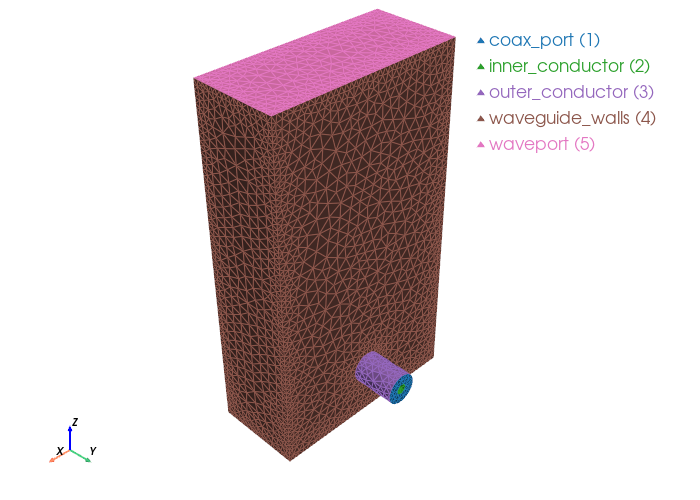
view_mesh(filename, transparent_groups= "air_sphere__None")
Loading mesh file: coax_to_waveguide.msh
Groups to render transparent: air_sphere__None

Mesh loaded successfully with 2 cell blocks
Found 7748 triangles total
Physical group tags in mesh: {1: 'coax_port', 2: 'inner_conductor', 3: 'outer_conductor', 4: 'waveguide_walls', 5: 'waveport'}
Generating the Palace Configuration File#
Finally, we assemble the simulation parameters into a JSON configuration file. This file serves as the definitive input for Palace.
palace_config = {
    "Problem": {
        "Type": "Driven",
        "Verbose": 2,
        "Output": "postpro/coax2waveguide"
    },
    "Model": {
        "Mesh": "coax_to_waveguide.msh",
        "L0": 1e-3,
        "Refinement": {}
    },
    "Domains": {
        "Materials": [
            {
                "Attributes": [pg_map["waveguide_volume"]],
                "Permittivity": 1.0,
                "Permeability": 1.0
            },
            {
                "Attributes": [pg_map["dielectric"]],
                "Permittivity": 2.2,
                "Permeability": 1.0
            }
        ]
    },
    "Boundaries": {
        "PEC": {
            "Attributes": [pg_map["waveguide_surface"]] + [pg_map["outer_cyl"]] + [pg_map["probe"]]
        },
        "WavePort": [
            {
                "Index": 2,
                "Attributes": [pg_map["waveport"]],
                "Mode": 1,
                "Offset": 0.0
            },
            {
                "Index": 1,
                "Attributes": [pg_map["coax_port"]],
                "Mode": 1,
                "Offset": 0.0,
                "Excitation": True
            }
        ]
    },
    "Solver": {
        "Order": 2,
        "Device": "CPU",
        "Driven": {

            "MinFreq": 6.0,
            "MaxFreq": 12.0,
            "FreqStep": 0.1,
            "SaveStep": 2,
            "AdaptiveTol": 0.001
        },
        "Linear": {
            "Type": "Default",
            "KSPType": "GMRES",
            "Tol": 1e-08,
            "MaxIts": 200,
            "ComplexCoarseSolve": True
        }
    }
}

with open("coax_to_waveguide.json", 'w') as json_file:
    json.dump(palace_config, json_file, indent=4)

print(f"Palace config successfully generated: coax_to_waveguide.json")
Palace config successfully generated: coax_to_waveguide.json